Chapter 7 傾向スコア
傾向スコアは、コホート研究(横断研究)などで良く用いられる手法です。 コホート研究においても、暴露群と対照群を比較することがあります。 ランダム化比較試験と比べると、2群が必ずしも同じような属性を持っているとは限りません。 そのため、研究対象者の中から似たような人々をマッチングさせて、指定した属性が同じようになるようにサブセットを作ります。
傾向スコアを求めるには、ロジステイック回帰を用います。
ln OR\(_y\) = \(\alpha\) + ln OR\(_1\) \(\times\) \(x_1\) + ln OR\(_2\) \(x_2\) + \(\cdots\)
対数の底は自然対数 \(e\)。
OR \(_i\):
- \(x_i\) が2値変数の時(ex. 男=0 or 女=1)、\(y\) の男に対する女のオッズ比。
- \(x_i\) が連続変数の時、\(y\) の \(x_i\) が1大きくなる時のオッズ比。
OR\(_y\) は、アウトカムの発生オッズ比
ln OR\(_y\) を傾向スコアとします。 このため、傾向スコアは0から1の間の数値をとります。
7.1 傾向スコアの進め方
- 通常通りに2群を比較
- 指定した説明変数で傾向スコアを計算
- 傾向スコアが近いもの同士をマッチング
- マッチングで作成された2群の2で使わなかった説明変数を比較
また、ここでできた2群を、通常通り統計解析することも可能です。
7.2 論文 Masaki S and Kawamoto T (2019)
傾向スコアを使用した論文に、以下のものがあります。
Masaki S & Kawamoto T (2019) Comparison of long-term outcomes between enteral nutrition via gastrostomy and total parenteral nutrition in older persons with dysphagia: A propensity-matched cohort study. PLoS One, 14(10), e0217120.
嚥下障害のある高齢者における人工栄養では、経皮的内視鏡下胃瘻造設術(PEG)が代表的です。しかしながら、日本では近年PEGが不要な延命と見なされていることもあり、(TPN)が不適切に選択されることもあります。そこで、PEGまたはTPNを受けた高齢嚥下障害患者の生存期間などを調査しました。その際に、アウトカム以外の評価項目を用いて1対1の傾向スコアマッチングをいました。
PEG(n=180)またはTPN(n=73)を受けた253名の患者を確認し、傾向スコアマッチングにより55組が作成されました。生存期間はPEG群のほうが有意に長い結果となりました(中央値、317日対195日、P = 0.017)。PEG群の方が重症肺炎 (pneumonia) の発生率が高く、逆にTPN群の方が敗血症 (sepsis) の発生率が低かった結果となりました。
この研究でもRが使われているようですが、今回は論文で使われているのとは違うパッケージを使用します。論文のサイトからデータがダウンロードできるようになっています。では、データをダウンロード、解凍した後、以下のコードでデータを読み込んでみましょう。
7.3 xlsx データの読み込み
library(readxl)
dfPropensityScore <- read_excel("Dataset_PEG_TPN_Dryad.xlsx")dfPropensityScore$PEG <- factor(dfPropensityScore$PEG,
levels = c(1,0),
labels = c("PEG","TPN"))
dfPropensityScore$PORT <- factor(dfPropensityScore$PORT)
dfPropensityScore$NTCVC <- as.factor(dfPropensityScore$`NT-CVC`)
dfPropensityScore$PICC <- as.factor(dfPropensityScore$PICC)
dfPropensityScore$sex <- as.factor(dfPropensityScore$sex)
dfPropensityScore$CI <- as.factor(dfPropensityScore$CI)
dfPropensityScore$dement <- as.factor(dfPropensityScore$dement)
dfPropensityScore$NMD <- as.factor(dfPropensityScore$NMD)
dfPropensityScore$asp <- as.factor(dfPropensityScore$asp)
dfPropensityScore$IHD <- as.factor(dfPropensityScore$IHD)
dfPropensityScore$lung <- as.factor(dfPropensityScore$lung)
dfPropensityScore$liver <- as.factor(dfPropensityScore$liver)
dfPropensityScore$CKD <- as.factor(dfPropensityScore$CKD)R の解説書では、tidyverse を使って型変換を行うことが多いようです。 tidyverse(dplyr) を使うと、このようになります。
library(dplyr)
dfPropensityScore <- dfPropensityScore %>%
        mutate(PEG = factor(PEG,
                            levels = c(1,0),
                            labels = c("PEG","TPN")
                            ))
7.4 表1の作成
library(tableone)
CreateTableOne(data = dfPropensityScore,
               strata="PEG",
               vars=c("PORT","NTCVC","PICC", "age", "sex","CI","dement","NMD","asp","IHD","CHF","lung","liver","CKD","Alb", "TLC", "TC", "Hb", "CRP"),
               factorVars=c("PORT","NTCVC","PICC", "sex","CI","dement","NMD","asp","IHD","CHF","lung","liver","CKD"))
## Stratified by PEG
## PEG TPN p test
## n 180 73
## PORT = 1 (%) 0 ( 0.0) 28 (38.4) <0.001
## NTCVC = 1 (%) 0 ( 0.0) 26 (35.6) <0.001
## PICC = 1 (%) 0 ( 0.0) 19 (26.0) <0.001
## age (mean (SD)) 81.56 (9.84) 86.77 (6.72) <0.001
## sex = 1 (%) 109 (60.6) 45 (61.6) 0.985
## CI = 1 (%) 107 (59.4) 26 (35.6) 0.001
## dement = 1 (%) 57 (31.7) 45 (61.6) <0.001
## NMD = 1 (%) 10 ( 5.6) 4 ( 5.5) 1.000
## asp = 1 (%) 73 (40.6) 21 (28.8) 0.106
## IHD = 1 (%) 31 (17.2) 16 (21.9) 0.489
## CHF = 1 (%) 70 (38.9) 37 (50.7) 0.114
## lung = 1 (%) 12 ( 6.7) 7 ( 9.6) 0.592
## liver = 1 (%) 9 ( 5.0) 6 ( 8.2) 0.491
## CKD = 1 (%) 29 (16.1) 24 (32.9) 0.005
## Alb (mean (SD)) 3.24 (0.57) 2.82 (0.53) <0.001
## TLC (mean (SD)) 1383.84 (713.18) 1203.11 (682.95) 0.073
## TC (mean (SD)) 160.19 (38.06) 145.58 (43.21) 0.009
## Hb (mean (SD)) 11.29 (1.90) 10.21 (2.10) <0.001
## CRP (mean (SD)) 2.03 (2.77) 2.92 (3.04) 0.0267.5 MathcIt
まず、欠測値があるため、論文では多重代入法で代入していました。論文では rms ライブラリを使用したとありましたが、ここでは mice を使用します。
なお、当初はデータフレーム dfPropensityScore を直接操作しようとしましたが、以下のようなエラーが出てきました。
 iter imp variable
  1   1  TLC eval(predvars, data, env) でエラー:  オブジェクト 'NT' がありません
そこで、欠測値 (NA) がある列と関連すると思われる列だけを抽出して、代入を行い、データフレーム dfPropensityScore に戻すという処理を行いました。
library(mice)
# micePS <- mice(dfPropensityScore)
# dfPropensityScore <- complete(micePS, 1)

dfTemp <- dfPropensityScore[c("ID", "TLC", "TC", "age", "sex", "Alb", "Hb", "CRP")]
names(dfTemp) <- c("ID2", "TLC2", "TC2", "age2", "sex2", "Alb2", "Hb2", "CRP2")
micePS <- mice(dfTemp)
##
## iter imp variable
## 1 1 TLC2 TC2
## 1 2 TLC2 TC2
## 1 3 TLC2 TC2
## 1 4 TLC2 TC2
## 1 5 TLC2 TC2
## 2 1 TLC2 TC2
## 2 2 TLC2 TC2
## 2 3 TLC2 TC2
## 2 4 TLC2 TC2
## 2 5 TLC2 TC2
## 3 1 TLC2 TC2
## 3 2 TLC2 TC2
## 3 3 TLC2 TC2
## 3 4 TLC2 TC2
## 3 5 TLC2 TC2
## 4 1 TLC2 TC2
## 4 2 TLC2 TC2
## 4 3 TLC2 TC2
## 4 4 TLC2 TC2
## 4 5 TLC2 TC2
## 5 1 TLC2 TC2
## 5 2 TLC2 TC2
## 5 3 TLC2 TC2
## 5 4 TLC2 TC2
## 5 5 TLC2 TC2dfTemp <- complete(micePS, 1)
dfPropensityScore <- cbind(dfPropensityScore, dfTemp)次に、傾向スコアマッチングを実行します。
library("MatchIt")
library("optmatch")
## The optmatch package has an academic license. Enter relaxinfo() for more information.miPropensityScore <- matchit(
formula = PEG ~ age + sex + CI + dement + NMD + asp + IHD + CHF + lung + liver + CKD + Alb + TLC2 + TC2 + Hb + CRP,
data = dfPropensityScore,
method = "nearest",
distance = "glm",
caliper = 0.05,
ratio = 1)
summary(miPropensityScore)##
## Call:
## matchit(formula = PEG ~ age + sex + CI + dement + NMD + asp +
## IHD + CHF + lung + liver + CKD + Alb + TLC2 + TC2 + Hb +
## CRP, data = dfPropensityScore, method = "nearest", distance = "glm",
## caliper = 0.05, ratio = 1)
##
## Summary of Balance for All Data:
## Means Treated Means Control Std. Mean Diff. Var. Ratio eCDF Mean
## distance 0.4613 0.2185 1.2114 1.0783 0.3163
## age 86.7671 81.5556 0.7753 0.4663 0.1121
## sex0 0.3836 0.3944 -0.0224 . 0.0109
## sex1 0.6164 0.6056 0.0224 . 0.0109
## CI0 0.6438 0.4056 0.4976 . 0.2383
## CI1 0.3562 0.5944 -0.4976 . 0.2383
## dement0 0.3836 0.6833 -0.6165 . 0.2998
## dement1 0.6164 0.3167 0.6165 . 0.2998
## NMD0 0.9452 0.9444 0.0033 . 0.0008
## NMD1 0.0548 0.0556 -0.0033 . 0.0008
## asp0 0.7123 0.5944 0.2604 . 0.1179
## asp1 0.2877 0.4056 -0.2604 . 0.1179
## IHD0 0.7808 0.8278 -0.1135 . 0.0470
## IHD1 0.2192 0.1722 0.1135 . 0.0470
## CHF 0.5068 0.3889 0.2359 . 0.1180
## lung0 0.9041 0.9333 -0.0993 . 0.0292
## lung1 0.0959 0.0667 0.0993 . 0.0292
## liver0 0.9178 0.9500 -0.1172 . 0.0322
## liver1 0.0822 0.0500 0.1172 . 0.0322
## CKD0 0.6712 0.8389 -0.3569 . 0.1677
## CKD1 0.3288 0.1611 0.3569 . 0.1677
## Alb 2.8233 3.2417 -0.7854 0.8686 0.1381
## TLC2 1209.5945 1383.8361 -0.2584 0.8940 0.0949
## TC2 145.8082 160.8000 -0.3490 1.1788 0.0997
## Hb 10.2096 11.2922 -0.5161 1.2193 0.1239
## CRP 2.9194 2.0327 0.2920 1.2037 0.1416
## eCDF Max
## distance 0.5134
## age 0.2553
## sex0 0.0109
## sex1 0.0109
## CI0 0.2383
## CI1 0.2383
## dement0 0.2998
## dement1 0.2998
## NMD0 0.0008
## NMD1 0.0008
## asp0 0.1179
## asp1 0.1179
## IHD0 0.0470
## IHD1 0.0470
## CHF 0.1180
## lung0 0.0292
## lung1 0.0292
## liver0 0.0322
## liver1 0.0322
## CKD0 0.1677
## CKD1 0.1677
## Alb 0.3241
## TLC2 0.2117
## TC2 0.1954
## Hb 0.2868
## CRP 0.3149
##
##
## Summary of Balance for Matched Data:
## Means Treated Means Control Std. Mean Diff. Var. Ratio eCDF Mean
## distance 0.3962 0.3956 0.0030 1.0074 0.0049
## age 86.5000 86.7115 -0.0315 1.2038 0.0205
## sex0 0.3846 0.3654 0.0395 . 0.0192
## sex1 0.6154 0.6346 -0.0395 . 0.0192
## CI0 0.6346 0.6346 0.0000 . 0.0000
## CI1 0.3654 0.3654 0.0000 . 0.0000
## dement0 0.4038 0.4038 0.0000 . 0.0000
## dement1 0.5962 0.5962 0.0000 . 0.0000
## NMD0 0.9615 0.9423 0.0845 . 0.0192
## NMD1 0.0385 0.0577 -0.0845 . 0.0192
## asp0 0.6538 0.6154 0.0850 . 0.0385
## asp1 0.3462 0.3846 -0.0850 . 0.0385
## IHD0 0.8269 0.7885 0.0930 . 0.0385
## IHD1 0.1731 0.2115 -0.0930 . 0.0385
## CHF 0.4615 0.5192 -0.1154 . 0.0577
## lung0 0.9423 0.9038 0.1306 . 0.0385
## lung1 0.0577 0.0962 -0.1306 . 0.0385
## liver0 0.9423 0.9231 0.0700 . 0.0192
## liver1 0.0577 0.0769 -0.0700 . 0.0192
## CKD0 0.7308 0.7308 0.0000 . 0.0000
## CKD1 0.2692 0.2692 0.0000 . 0.0000
## Alb 2.9308 2.9385 -0.0144 0.7344 0.0276
## TLC2 1223.1654 1167.2808 0.0829 1.6231 0.1018
## TC2 142.5577 145.9808 -0.0797 1.3955 0.0458
## Hb 10.4135 10.3115 0.0486 1.0280 0.0278
## CRP 3.0858 2.6410 0.1465 0.9407 0.0944
## eCDF Max Std. Pair Dist.
## distance 0.0385 0.0140
## age 0.0577 0.9985
## sex0 0.0192 0.9887
## sex1 0.0192 0.9887
## CI0 0.0000 0.4231
## CI1 0.0000 0.4231
## dement0 0.0000 0.3846
## dement1 0.0000 0.3846
## NMD0 0.0192 0.4225
## NMD1 0.0192 0.4225
## asp0 0.0385 0.9346
## asp1 0.0385 0.9346
## IHD0 0.0385 0.7438
## IHD1 0.0385 0.7438
## CHF 0.0577 0.8078
## lung0 0.0385 0.5225
## lung1 0.0385 0.5225
## liver0 0.0192 0.3501
## liver1 0.0192 0.3501
## CKD0 0.0000 0.4231
## CKD1 0.0000 0.4231
## Alb 0.1346 1.0614
## TLC2 0.2308 0.9709
## TC2 0.1538 0.9223
## Hb 0.0962 0.9470
## CRP 0.2500 0.9445
##
## Percent Balance Improvement:
## Std. Mean Diff. Var. Ratio eCDF Mean eCDF Max
## distance 99.8 90.2 98.4 92.5
## age 95.9 75.7 81.7 77.4
## sex0 -76.7 . -76.7 -76.7
## sex1 -76.7 . -76.7 -76.7
## CI0 100.0 . 100.0 100.0
## CI1 100.0 . 100.0 100.0
## dement0 100.0 . 100.0 100.0
## dement1 100.0 . 100.0 100.0
## NMD0 -2426.9 . -2426.9 -2426.9
## NMD1 -2426.9 . -2426.9 -2426.9
## asp0 67.4 . 67.4 67.4
## asp1 67.4 . 67.4 67.4
## IHD0 18.1 . 18.1 18.1
## IHD1 18.1 . 18.1 18.1
## CHF 51.1 . 51.1 51.1
## lung0 -31.6 . -31.6 -31.6
## lung1 -31.6 . -31.6 -31.6
## liver0 40.3 . 40.3 40.3
## liver1 40.3 . 40.3 40.3
## CKD0 100.0 . 100.0 100.0
## CKD1 100.0 . 100.0 100.0
## Alb 98.2 -119.1 80.0 58.5
## TLC2 67.9 -332.1 -7.2 -9.0
## TC2 77.2 -102.6 54.0 21.2
## Hb 90.6 86.1 77.6 66.5
## CRP 49.8 67.0 33.3 20.6
##
## Sample Sizes:
## Control Treated
## All 180 73
## Matched 52 52
## Unmatched 128 21
## Discarded 0 0関数
- matchit: ライブラリ MatchiIt の関数
引数
- formula: ロジスティック回帰のモデル。なお、‘=’ は引数をとる時に使うため、モデル内の ‘=’ は ‘~’ と書きます。
- data: データフレーム
- method: マッチングの方法。より厳密な “exact” や、サンプルサイズが大きくなる “full” (ただし、1:1にはなりません)などがあります。
- distance
- caliper: distance の数値でマッチングを行う際に許容される差の閾値。
- ratio: 両群のサンプルサイズの比率。
dfPSMatched <- match.data(miPropensityScore)CreateTableOne(data = dfPSMatched,
strata="PEG",
vars=c("PORT","NTCVC","PICC", "age", "sex","CI","dement","NMD","asp","IHD","CHF","lung","liver","CKD","Alb", "TLC", "TC", "Hb", "CRP"),
factorVars=c("PORT","NTCVC","PICC", "sex","CI","dement","NMD","asp","IHD","CHF","lung","liver","CKD"))## Stratified by PEG
## PEG TPN p test
## n 52 52
## PORT = 1 (%) 0 ( 0.0) 19 (36.5) <0.001
## NTCVC = 1 (%) 0 ( 0.0) 20 (38.5) <0.001
## PICC = 1 (%) 0 ( 0.0) 13 (25.0) <0.001
## age (mean (SD)) 86.71 (6.68) 86.50 (7.33) 0.878
## sex = 1 (%) 33 (63.5) 32 (61.5) 1.000
## CI = 1 (%) 19 (36.5) 19 (36.5) 1.000
## dement = 1 (%) 31 (59.6) 31 (59.6) 1.000
## NMD = 1 (%) 3 ( 5.8) 2 ( 3.8) 1.000
## asp = 1 (%) 20 (38.5) 18 (34.6) 0.839
## IHD = 1 (%) 11 (21.2) 9 (17.3) 0.804
## CHF = 1 (%) 27 (51.9) 24 (46.2) 0.695
## lung = 1 (%) 5 ( 9.6) 3 ( 5.8) 0.713
## liver = 1 (%) 4 ( 7.7) 3 ( 5.8) 1.000
## CKD = 1 (%) 14 (26.9) 14 (26.9) 1.000
## Alb (mean (SD)) 2.94 (0.57) 2.93 (0.49) 0.942
## TLC (mean (SD)) 1167.28 (543.59) 1195.02 (700.51) 0.824
## TC (mean (SD)) 145.51 (33.84) 142.18 (43.02) 0.677
## Hb (mean (SD)) 10.31 (1.87) 10.41 (1.89) 0.783
## CRP (mean (SD)) 2.64 (3.37) 3.09 (3.27) 0.496library(survival)
library(survminer)
objSurv <- survfit( Surv(survival,status) ~ PEG,
data = dfPSMatched)
ggsurvplot(objSurv,
data = dfPSMatched,
risk.table = TRUE,
pval = TRUE,
conf.int = TRUE,
risk.table.y.text.col = TRUE)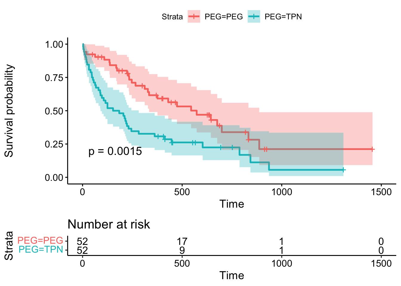
dfPSMatched$oral <- as.factor(dfPSMatched$oral)
dfPSMatched$home <- as.factor(dfPSMatched$home)
dfPSMatched$pneumo <- as.factor(dfPSMatched$pneumo)
dfPSMatched$sepsis <- as.factor(dfPSMatched$sepsis)

CreateTableOne(data = dfPSMatched,
               strata="PEG",
               vars=c("oral", "home", "pneumo", "sepsis"),
               factorVars=c("oral", "home", "pneumo", "sepsis"))
## Stratified by PEG
## PEG TPN p test
## n 52 52
## oral = 1 (%) 4 ( 7.7) 3 ( 5.8) 1.000
## home = 1 (%) 10 (19.2) 6 (11.5) 0.415
## pneumo = 1 (%) 18 (34.6) 11 (21.6) 0.210
## sepsis = 1 (%) 6 (11.5) 17 (33.3) 0.016